
PPP Financial Modeling
Jun 04, 2025
PPP Financial Modeling: Purpose, Uses, and Toll Road Example
A PPP financial model is a detailed spreadsheet that integrates all project inputs (capex, opex, demand, tariffs, financing, etc.) to project cash flows over the concession life. Its purpose is to test viability and guide structuring: demonstrating whether the project can attract private finance and meet stakeholder objectives. For example, an Asian Development Bank guide notes that a financial model “simulates the financial results of the project by demonstrating anticipated cash flow under different scenarios,” reflecting assumptions on risks, tariffs and financing. In practice, the model serves as the financial “base case” of the Special Purpose Vehicle (SPV), incorporating all expected investments, revenues, costs, taxes, and parameters such as debt/equity costs and inflation. In short, it provides the economic blueprint of the PPP: quantifying how cash enters and leaves the project, testing profitability, and enabling analyses of alternatives or policy choices.
The objectives of a PPP financial model include: (1) assessing commercial viability (can private investors earn their required returns?), (2) checking bankability (do lenders see sufficient cash to repay debt on schedule?), (3) informing value-for-money (VfM) comparisons (PPP vs traditional procurement), and (4) evaluating fiscal impact (affordability for the government). For instance, one PPP procurement guide highlights that the model lets decision-makers explore different tariff levels and subsidy regimes and “understand how lenders, partners, and consumers may perceive the project”. It explicitly shows project revenues, operating costs, debt service and balance sheet metrics (e.g. DSCR, cash sweeps) under the PPP structure. In summary, a good PPP financial model is the “critical component” in structuring a project, used by both public and private parties to predict cash flows and test viability.
Role in Feasibility and Decision-Making
In early feasibility and screening studies, the financial model is developed (often by government advisors) to test whether a PPP is feasible and affordable. At this stage the deliverable is a “risk-adjusted PPP financial model” that analyzes the project’s financial soundness under the preferred solution. It incorporates detailed cost projections (construction, maintenance, operation) and revenue forecasts, and it quantifies whether these cash flows can cover financing costs. Critically, the model in feasibility also estimates public-sector impacts: incremental tax revenues, increased recurrent costs, budget obligations and any required subsidies. For example, PPP guidelines require the model to include the “impact of the project on public sector/government finances,” considering factors like incremental taxes and recurrent expenditures.
As the project moves to appraisal and bidding, the financial model guides final decisions. It underpins the commercial viability and value-for-money analysis: comparing the PPP option against the traditional (public-financed) route. In value-for-money assessments, a “Public Sector Comparator” (PSC) is built using similar spreadsheet modeling to represent the cost if the government delivered the project directly. The PPP model is then compared to the PSC to see which yields a lower whole-life cost or better returns. At the tender stage, prospective bidders each build their own models (“bid models”) to price their offers, but the government uses a core model to evaluate bids. After contract award, the winning bid’s model effectively becomes the contract baseline. Even post-financial close, both the private partner and the authority use the model to monitor performance and adjust for changes (e.g. unforeseen cost overruns or traffic shortfalls).
Step-by-Step Guide to Building a PPP Financial Model
-
Define Project Scope and Outputs. Specify the concession length, construction schedule, and technical standards. Clarify the services and outputs required (e.g. road capacity, toll policy). This establishes the time frame and units for the model.
-
Estimate Direct Costs. Identify all capital expenditures (CAPEX) and operating/maintenance costs. Direct capital costs include construction, land, equipment, design and implementation (labor, management, professional fees). Direct operating costs cover routine expenses (personnel, fuel, consumables, periodic maintenance). Include costs over the asset life (e.g. major rehabilitation, asset replacement) in the model when they occur.
-
Identify Indirect and Overhead Costs. Allocate project overheads (management, insurance, office, contingencies) that can be apportioned to the service. These are captured as indirect costs in the model.
-
Forecast Revenues. Project demand (e.g. vehicle traffic, service usage) and pricing assumptions. For a toll road, this means estimating peak and base traffic volumes and toll rates by year, then computing annual toll revenue. (Any shadow-toll or availability payments must also be modeled.) Revenues should be linked to realistic assumptions or benchmarks.
-
Set Macro and Financial Assumptions. Document key assumptions in a separate input sheet: inflation rates, traffic growth, toll escalation, interest rates, exchange rates, income tax rates, discount rates, construction cost escalation, etc. These assumptions drive the base-case projections.
-
Build the Base-Case Cash Flow. Using the above inputs, construct a year-by-year discounted cash flow model. Calculate annual revenues, subtract operating costs to get EBITDA (or CFADS – cash flow available for debt service), then apply financing (interest and principal) to find cash flow to equity. Also maintain a balance sheet if needed. The goal is to produce the project’s net cash flow profile over the full concession.
-
Develop a Risk Matrix. Identify project risks (construction delays, cost overruns, demand shortfall, policy risk, etc.), quantify their impacts, and decide who bears each risk. Prepare a risk register as part of the feasibility exercise.
-
Incorporate Risk Adjustments. Modify the base model to include risk contingencies: add cost buffers or insurance premiums, adjust revenues for downside demand scenarios, etc. This “risk-adjusted” model shows realistic worst-case or expected scenarios.
-
Finalize Financing Structure. Specify the funding plan: the debt‐equity split, debt terms (interest rate, tenor, grace periods), and the equity return requirements. Calculate annual debt service (interest + principal) and set debt-service coverage constraints. For example, ensure the target Debt Service Coverage Ratio (DSCR) (cash flow/debt service) meets typical lender criteria (often ≥1.1–1.3). Incorporate debt service reserve accounts (DSRA) if required.
-
Calculate Output Metrics and Perform Sensitivity Analysis. Compute the key project metrics: Net Present Value (NPV) of equity cash flows, Equity Internal Rate of Return (Equity IRR), Project IRR (including debt), Debt Service Coverage Ratio (DSCR), Loan Life Coverage Ratio (LLCR), etc. By definition, IRR is the discount rate that makes NPV zero. Finally, run sensitivity and scenario analyses: vary major assumptions (±10–20% in traffic, tolls, CAPEX, OPEX) to see how IRR, NPV, and DSCR respond. This reveals whether the project remains viable under adverse conditions.
Worked Example: Toll Road PPP Financial Model
Assumptions: Consider a hypothetical 100‑km toll road PPP concession. The key assumptions might be:
| Parameter | Value (Example) |
|---|---|
| Concession Term (incl. 3‑yr build) | 23 years (3Y build + 20Y operate) |
| Construction Period | 3 years (Years 0–2) |
| Total CAPEX | $300 million (evenly spread) |
| Opening Year | Year 3 (first toll revenues Year 4) |
| Initial Daily Traffic | 25,000 vehicles (year 4) |
| Traffic Growth Rate | 3.0% per year |
| Initial Toll Rate | $4.00 per vehicle |
| Toll Escalation (CPI) | 2.0% per year |
| Initial O&M Cost (annual) | $10 million (year 4) |
| O&M Cost Growth | 2.0% per year (CPI) |
| Debt Ratio | 70% debt / 30% equity |
| Interest Rate (nominal) | 6.0% per annum (fixed) |
| Debt Term (amortization) | 15 years (Years 4–18) |
| Inflation (CPI) | 2.0% per year |
| Discount Rate (Equity) | 10.0% (for NPV calc) |
Based on these inputs, the model projects yearly toll revenue = (traffic×365×toll rate), escalating over 20 operating years. Operating costs (O&M) rise with inflation. Debt is drawn during construction and repaid over 15 years once tolls start.
Financial Calculations: During Years 0–2 (construction), the project incurs $300M CAPEX (financed 70% debt, 30% equity). Interest accrues on drawn debt and is capitalized. In Year 3 the road opens, and from Years 4–23 toll revenue flows in. Each year’s EBITDA = Revenue – O&M – major maintenance. From this, debt service (interest+principal) is paid, with any surplus as cash to equity.
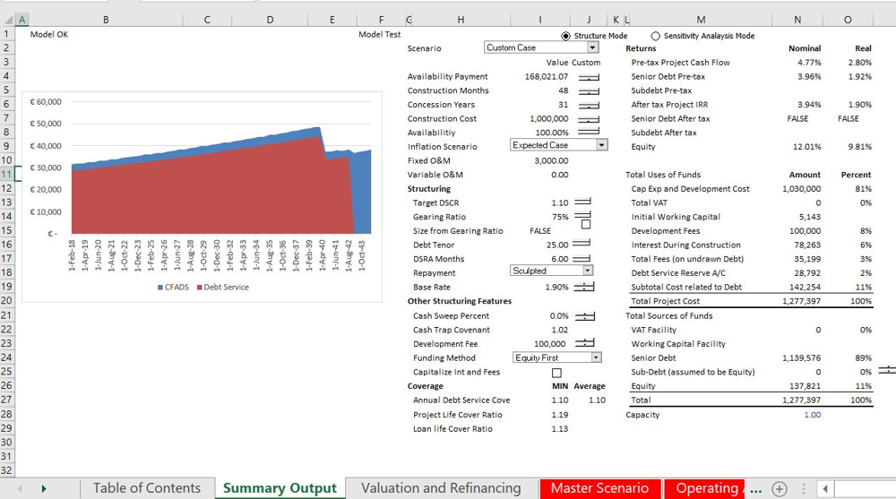
Figure: Example output from a toll‑road PPP model (blue = cash available for debt; red = debt service). The model computes financing metrics (right panel) and key ratios. The chart above illustrates typical cash flows: debt service (red) peaks early and then falls off, while cash available (blue) grows as traffic builds. In this example the target DSCR (minimum) is set at 1.10, and actual DSCR quickly exceeds this as revenue ramps up. The summary (right panel) shows Equity IRR ≈12.0%, Project IRR ≈3.9%, and a steady DSCR above ~1.2 once operations stabilize.
Key Results: Under these assumptions, the model yields a positive NPV and attractive returns. For instance:
-
Equity IRR: ≈12.0% (nominal, ~10% real) – above a typical 10% hurdle, indicating sufficient return.
-
Project IRR (pre-tax): ≈3.9% (lower since it includes debt leverage).
-
NPV (Equity, 10%): ≈$29 million (positive NPV confirms viability at the chosen discount rate).
-
Average DSCR: ≈1.3 (i.e. cash covers debt by ~1.3× on average). Lenders see this as acceptable – a higher DSCR implies lower risk.
-
Minimum DSCR: ≈0.9 in Year 1 (ramp-up year), but this is typically managed by capitalizing interest or equity top-ups.
-
Debt/Equity: 70/30 (consistent with project finance norms).
-
Loan Life Coverage Ratio (LLCR): ≈1.84 (present value of cash flows over debt term / outstanding debt).
These outputs illustrate global best practice: building conservative assumptions, matching debt tenor shorter than concession (creating a “tail” buffer), and reporting both project and equity IRRs along with coverage ratios. The IRR and NPV measure whether investors get a competitive return, while DSCR and LLCR ensure lenders will be repaid on time. (Formulas: IRR is the discount rate making NPV=0; NPV is the sum of discounted cash flows beyond the discount rate). Sensitivity analysis would vary toll growth or costs (e.g. –20% traffic, +20% capex) to confirm the project remains bankable under stress.
Stakeholder Perspectives
The model supports both private and public decision-makers. From the private investor’s viewpoint, the focus is on returns and risk. An equity IRR above the sector’s required return and DSCR comfortably above minimum thresholds signal a viable, “bankable” deal.. For lenders, the DSCR (cashflow/debt service) is crucial – a higher DSCR means more cushion. In our example the target DSCR of 1.10 is exceeded by actual cash flows, giving lenders confidence that debt can be serviced even if revenues dip.
From the public sector’s perspective, the model quantifies value-for-money and affordability. In a user-pay PPP (toll road), the government pays nothing directly but earns ancillary benefits. The model can show increased tax receipts (fuel taxes, vehicle taxes) and saved maintenance costs on parallel routes. It also highlights any fiscal support needed (e.g. minimum-traffic guarantees or subsidies). By comparing to a Public Sector Comparator (i.e. the model of a traditionally financed project), authorities can see if PPP offers lower long-term cost. As PPP guidelines emphasize, the government uses the model to assess economic and fiscal feasibility: ensuring the project meets social objectives without untenable cost to the budget. For example, the model will show if tolls remain affordable (considering inflation) and if incremental budgetary obligations (counterparts or guarantees) are acceptable. In short, the model ensures both the private partner and the public side have a clear, quantifiable basis for their decision.
Sources
This guide is based on leading PPP practice from international agencies and toolkits (ADB, World Bank/PPPIRC, PPP certification guides), incorporating global lessons in financial structuring and analysis. Each assumption and result should be documented and stress-tested to meet those best-practice standards.
The PPP Alliance is an independent body of knowledge for the advancement of Public-Private Partnership knowledge and best practices.
Interested in joining the community? Become a member today.
Stay connected with news and updates!
Join our mailing list to receive the latest news and updates from our team.
Don't worry, your information will not be shared.
We hate SPAM. We will never sell your information, for any reason.
